1. Learning Objectives

• Plot bar charts and line charts using the dataset.
• Construct historical shift features and window statistical features from time series data.
• Train and predict using the LightGBM model.

2. GBDT and LightGBM

GBDT (Gradient Boosting Decision Tree) is a long-standing model in machine learning. Its main idea is to iteratively train weak classifiers (decision trees) to obtain an optimal model, which has advantages such as good training performance and resistance to overfitting.

GBDT is widely used in industry, commonly applied to tasks like multi-class classification, click-through rate prediction, and search ranking. It is also a powerful tool in data mining competitions. According to statistics, more than half of the winning solutions on Kaggle are based on GBDT.

LightGBM (Light Gradient Boosting Machine) is a framework that implements the GBDT algorithm. It supports efficient parallel training, offers faster training speed, lower memory consumption, better accuracy, and can handle massive data with distributed support.

LightGBM also includes models like random forest and logistic regression. Its commonly used in binary classification, multi-class classification, and ranking scenarios.

For example, in personalized product recommmendation, click-through rate prediction models are often needed. User behavior data (clicks, exposures without clicks, purchases) is used as training data to predict the probability of a user clicking or purchasing. Features are extracted from user behavior and attributes, including:

• Categorical features: string type, e.g., gender (male/female).
• Item type: clothing, toys, electronics, etc.
• Numerical features: integer or float type, e.g., user activity level or product price.

3. Code

3.1 Required Modules

import numpy as np
import pandas as pd
import lightgbm as lgb
from sklearn.metrics import mean_squared_log_error, mean_absolute_error, mean_squared_error
import tqdm
import sys
import os
import gc
import argparse
import warnings
warnings.filterwarnings('ignore')

You may encounter an error.

Solution:

pip install lightgbm

3.2 Exploratory Data Analysis (EDA)

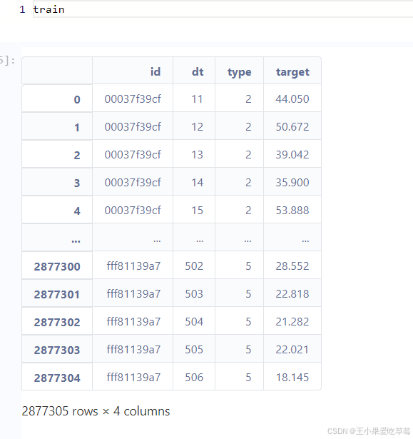
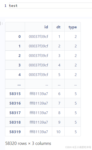
(1) Load training and test data, and display basic information.

train_df = pd.read_csv('./data/train.csv')
test_df = pd.read_csv('./data/test.csv')

Output:

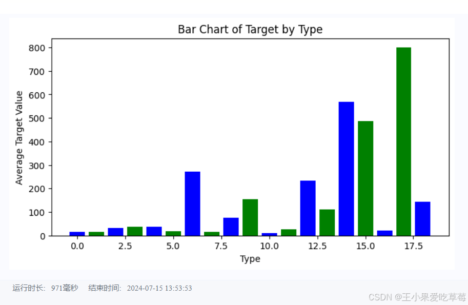
(2) Bar chart of average target by type.

import matplotlib.pyplot as plt
# Bar chart of average target by type
type_target = train_df.groupby('type')['target'].mean().reset_index()
plt.figure(figsize=(8, 4))
plt.bar(type_target['type'], type_target['target'], color=['blue', 'green'])
plt.xlabel('Type')
plt.ylabel('Average Target')
plt.title('Bar Chart of Target by Type')
plt.show()

Output:

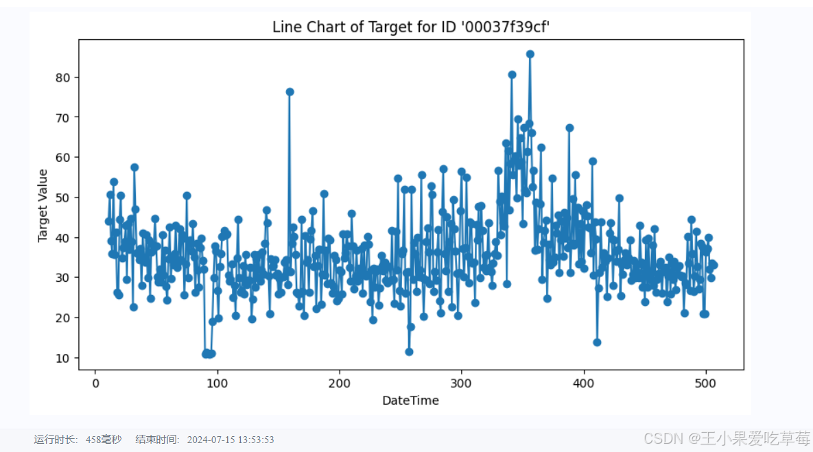
(3) Line chart of target over time for a specific ID.

specific_id = train_df[train_df['id'] == '00037f39cf']
plt.figure(figsize=(10, 5))
plt.plot(specific_id['dt'], specific_id['target'], marker='o', linestyle='-')
plt.xlabel('DateTime')
plt.ylabel('Target')
plt.title("Line Chart of Target for ID '00037f39cf'")
plt.show()

Output:

3.3 Feature Engineering

We construct historical shift features and window statistical features. Each feature has a rationale:

• Historical shift features: Capture information from previous time steps. For example, shift the target from time d-1 to d, and from d to d+1, creating a feature with a shift of one unit.

• Window statistical features: Aggregate statistics (mean, max, min, median, variance) over a sliding window of a certain size, reflecting recent changes. For instance, compute statistics of the three previous time steps to create a feature for the current time.

# Combine training and test data, then sort
data = pd.concat([test_df, train_df], axis=0, ignore_index=True)
data = data.sort_values(['id', 'dt'], ascending=False).reset_index(drop=True)

# Historical shifts: create features for lags 10 to 29
for i in range(10, 30):
    data[f'lag_{i}_target'] = data.groupby('id')['target'].shift(i)

# Window statistics: mean over a 3-step window using lag features
data['win3_mean_target'] = (data['lag_10_target'] + data['lag_11_target'] + data['lag_12_target']) / 3

# Split back into training and test sets
train_df = data[data['target'].notna()].reset_index(drop=True)
test_df = data[data['target'].isna()].reset_index(drop=True)

# Define feature columns
feature_cols = [col for col in data.columns if col not in ['id', 'target']]

3.4 Model Training and Test Prediction

We use the LightGBM model, a common baseline for data mining competitions, which provides stable scores even without extensive hyperparameter tuning.

Note the construction of training and validation sets: due to the time series nature, we split strictly chronologically. Here, we use data with dt >= 31 as training data and data with dt <= 30 as validation data. This avoids data leakage (using future data to predict the past).

def train_lightgbm(model, train_df, test_df, cols):
    # Split training and validation sets
    trn_x = train_df[train_df['dt'] >= 31][cols]
    trn_y = train_df[train_df['dt'] >= 31]['target']
    val_x = train_df[train_df['dt'] <= 30][cols]
    val_y = train_df[train_df['dt'] <= 30]['target']
    
    # Create LightGBM datasets
    train_data = model.Dataset(trn_x, label=trn_y)
    valid_data = model.Dataset(val_x, label=val_y)
    
    # LightGBM parameters
    params = {
        'boosting_type': 'gbdt',
        'objective': 'regression',
        'metric': 'mse',
        'min_child_weight': 5,
        'num_leaves': 2 ** 5,
        'lambda_l2': 10,
        'feature_fraction': 0.8,
        'bagging_fraction': 0.8,
        'bagging_freq': 4,
        'learning_rate': 0.05,
        'seed': 2024,
        'nthread': 16,
        'verbose': -1,
    }
    
    # Train the model
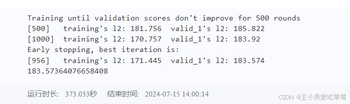
    model = lgb.train(params, train_data, num_boost_round=50000,
                      valid_sets=[train_data, valid_data],
                      callbacks=[lgb.early_stopping(500), lgb.log_evaluation(500)])
    
    # Predict on validation and test sets
    val_pred = model.predict(val_x, num_iteration=model.best_iteration)
    test_pred = model.predict(test_df[cols], num_iteration=model.best_iteration)
    
    # Evaluate offline score
    score = mean_squared_error(val_pred, val_y)
    print(f'Validation MSE: {score}')
    
    return val_pred, test_pred

val_pred, test_pred = train_lightgbm(lgb, train_df, test_df, feature_cols)

# Save results to local file
test_df['target'] = test_pred
test_df[['id', 'dt', 'target']].to_csv('submit.csv', index=False)

You may encounter an error:

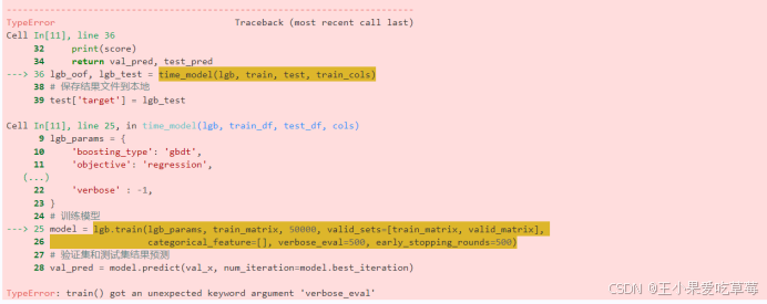
Solution: Downgrade LightGBM version.

pip install lightgbm==3.3.0

Output:

4. Links

Project experience link: https://aistudio.baidu.com/projectdetail/8151133

Submission link: submit the file to get scores.

My personal result: