Regression Algorithms

Regression is one of the most powerful tools in statistics. Supervised learning algorithms in machine learning are categorized into classification and regression algorithms, defined by whether the label distribution is discrete or continuous. Regression algorithms are used for predicting continuous distributions, targeting numerical samples. They allow predicting a numeric value given an input, which is an advancement over classification as it enables prediction of continuous data rather than just discrete class labels.

When regression analysis involves only one independent variable and one dependent variable, and their relationship can be approximated by a straight line, it is called simple linear regression analysis. If the analysis involves two or more independent variables and the relationship between the dependent and independent variables is linear, it is called multiple linear regression analysis. So, what are linear and nonlinear relationships?

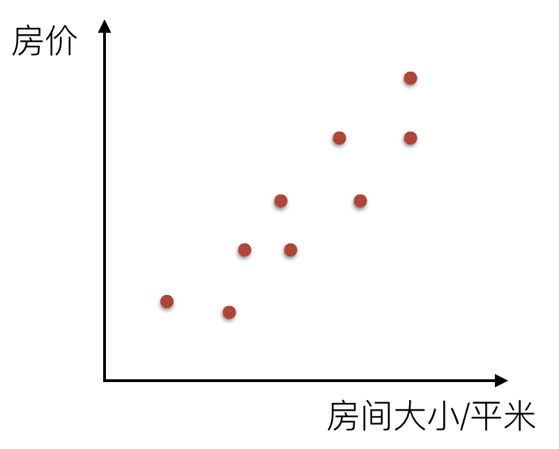
For example, in housing prices, there is a clear relationship between the size of a house and its price. Let X = house size, Y = house price. The points can be visualized in a coordinate system:

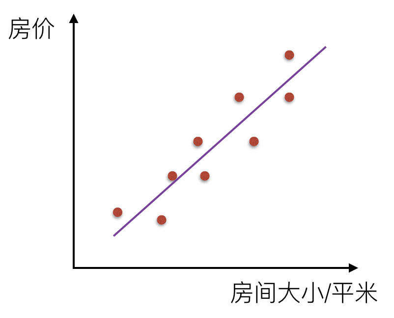
Describing this relationship with a straight line represents a linear relationship:

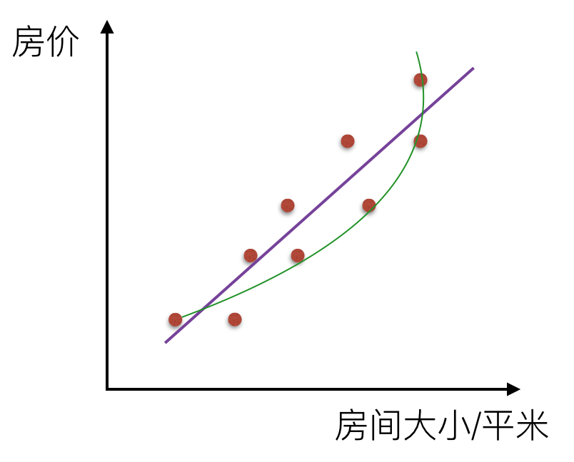
A curve represents a nonlinear relationship:

The goal of regression is to establish a regression equation (function) to predict target values. Solving regression involves finding the regression coefficients of this equation.

Linear Regression

Linear regression is defined as the expectation that the target value is a linear combination of the input variables. Linear models are simple in form and easy to model, yet they embody some important fundamental ideas in machine learning. Linear regression uses statistical regression analysis to determine the quantitative relationship between two or more variables and is widely applied.

Advantages: Easy to understand results, simple computation. Disadvantages: Poor fit for nonlinear data. Applicable data types: Numerical and nominal.

For univariate linear regression, e.g., predicting house price based on size: f(x) = w1*x + w0. The prediction can be made through the main parameter w1.

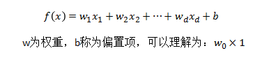
The general formula is:

For multivariate regression, e.g., evaluating melon quality: f(x) = w0 + 0.2color + 0.5stem + 0.3*sound, the value determines the melon's quality.

The general formula is:

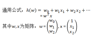
The weight vector W in linear models objectively expresses the importance of each attribute in prediction, giving linear models good interpretability. For "multi-feature prediction" (multiple linear regression), the goal is to obtain these W values, build a model, and predict test data. Simply put, we learn a linear model to predict real-valued output markers as accurately as possible.

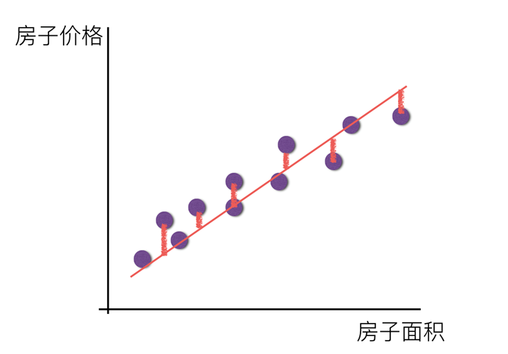
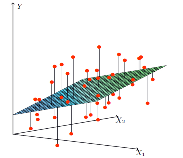
There is always some error between predicted results and true values.

Univariate error:

Multivariate error:

Loss Function

The loss function is an important concept throughout machine learning. Most machine learning algorithms have errors, and we need to describe this error explicitly and minimize it.

For linear regression models, the sum of squared distances between the model and data points is used as a measure of fit. The smaller the error, the better the fit. We aim to find the model that best matches f(x) to the true values. The error formula is to minimize the sum of squared differences between the model and data:

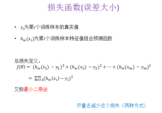
How to find W that minimizes the loss? (Goal: find W corresponding to the minimum loss)

Normal Equation (Not Required)

Visualization of loss function (univariate example):

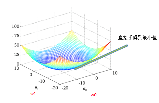
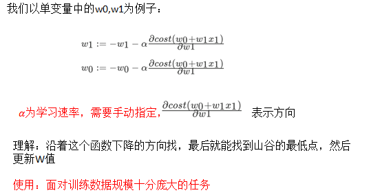
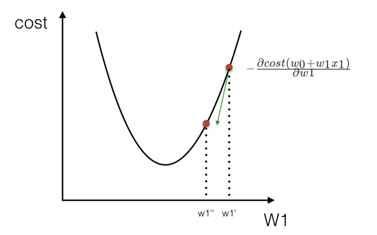
Gradient Descent (Understanding the Process)

Scikit-learn Linear Regression APIs

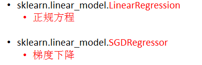
• sklearn.linear_model.LinearRegression(): Ordinary least squares linear regression.
  • coef_: Regression coefficients.
• sklearn.linear_model.SGDRegressor(): Linear model minimized via SGD.
  • coef_: Regression coefficients.

Linear Regression Example

1. Using scikit-learn's normal equation and gradient descent APIs.
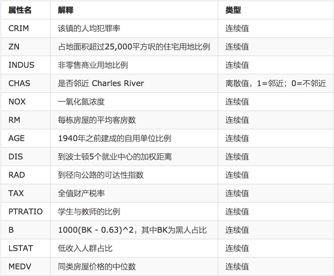
2. Analysis of the Boston housing dataset:
   • Load Boston housing data
   • Split data into training and test sets
   • Standardize training and test features
   • Predict housing prices using LinearRegression and SGDRegressor

Normal Equation

from sklearn import datasets
from sklearn.model_selection import train_test_split
from sklearn.preprocessing import StandardScaler
from sklearn.linear_model import LinearRegression
from sklearn.metrics import mean_squared_error

def predict_boston():
    """
    Predict Boston housing prices using linear regression.
    :return: None
    """
    dataset = datasets.load_boston()
    x_train, x_test, y_train, y_test = train_test_split(dataset.data, dataset.target, test_size=0.2)

    scaler = StandardScaler()
    x_train = scaler.fit_transform(x_train)
    x_test = scaler.transform(x_test)

    model = LinearRegression()
    model.fit(x_train, y_train)
    predictions = model.predict(x_test)
    print(predictions)

    print("True prices:", y_test)
    mse = mean_squared_error(y_test, predictions)
    print("Mean Squared Error:", mse)
    return None

if __name__ == '__main__':
    predict_boston()

Output:

[30.09 24.35 24.67 19.56 23.01 21.48 24.20 25.98 19.67 29.24 25.05 27.32 19.04 21.52  8.12 36.60 26.18 23.04  8.09 24.52 37.60 18.21 15.05 15.39 24.39 31.10 20.97 20.53 24.97 17.56 23.22 17.02 36.85  5.75 28.94 17.14 27.59 23.14 13.37 31.38 22.06 25.08 28.85 13.60 40.55 28.69 13.64 25.17 26.13 17.06  2.64 33.01 25.50 24.33 20.02 30.72 29.15 35.34 24.97 34.82 14.13 31.96 29.14 27.97 21.22 24.09  7.16 18.21 17.05 24.62 20.93 17.86 40.69 28.68 31.68 16.24 35.00 32.94 22.54 23.03 29.00 15.60 31.08 17.66 25.01 19.40 11.41 28.73 23.16  8.28 23.41 31.31 35.94 32.78  6.66 22.26 24.39 21.97  1.21 22.35 33.16 23.00]
True prices: [30.5 22.2 25.  19.4 26.4 24.5 21.9 22.2 22.2 25.  29.6 22.  17.8 21.4 11.9 50.  22.  23.   7.2 50.  44.  10.9 16.2 14.1 21.5 32.5 21.  20.1 25.  19.4 24.7 19.5 42.3  7.4 26.4 18.6 25.2 20.4 14.  31.5 23.2 50.  33.4 13.9 50.  24.4 10.9 29.8 22.8 18.1  8.1 32.  23.8 27.5 20.5 28.7 22.5 38.7 24.7 43.8  9.6 33.2 24.6 25.  20.1 23.4  7.  14.5 14.9 21.4 20.5 12.7 50.  24.3 27.   8.5 33.2 28.2 20.  20.8 22.9 13.3 28.4 19.4 24.6 16.7 16.3 22.8 21.7  5.  21.  29.9 33.3 33.1 10.4 22.4 23.1 18.7 17.9 20.2 31.7 25. ]
Mean Squared Error: 28.71

Gradient Descent

from sklearn import datasets
from sklearn.model_selection import train_test_split
from sklearn.preprocessing import StandardScaler
from sklearn.linear_model import SGDRegressor
from sklearn.metrics import mean_squared_error

def predict_boston():
    """
    Predict Boston housing prices using SGD.
    :return: None
    """
    dataset = datasets.load_boston()
    x_train, x_test, y_train, y_test = train_test_split(dataset.data, dataset.target, test_size=0.2)

    scaler = StandardScaler()
    x_train = scaler.fit_transform(x_train)
    x_test = scaler.transform(x_test)

    model = SGDRegressor()
    model.fit(x_train, y_train)
    predictions = model.predict(x_test)
    print("Gradient descent predictions:", predictions)
    mse = mean_squared_error(y_test, predictions)
    print("Gradient descent MSE:", mse)

if __name__ == '__main__':
    predict_boston()

Output:

Gradient descent predictions: [19.90 32.07 41.92 30.76 12.82 29.09 29.20 30.34 40.79 32.38 25.46 24.77 22.55 27.32 31.26 26.02 19.96 21.53 23.00 10.04 18.15 22.03 11.76  8.76 34.48 23.79 15.33 23.10 19.87 19.27 16.84 16.65 32.82 14.19 29.24 13.28 38.38 21.27 20.05 19.97 18.06 26.67 17.12 19.53 23.56 33.21 24.91 21.59 23.68 17.35 22.15  6.11 24.60 17.52 18.47 25.55 21.37 19.57 19.85 20.67 21.26  8.54 24.32 13.74 10.83 17.59 20.54  8.95 14.83 31.76 25.10 26.94 27.14 37.51 18.78 23.41 26.61 14.37 26.99 19.88 38.32 21.16 20.07 31.25 17.17 20.35 24.11 36.31 10.33 28.47 25.15 13.76 33.33 25.12 21.82 27.95 18.63 18.22 26.64 28.14 19.89 17.61]
Gradient descent MSE: 21.87

Regression Performance Evaluation

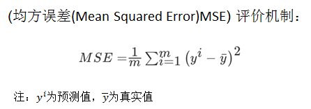
The scikit-learn API for regression evaluation is sklearn.metrics.mean_squared_error.

• mean_squared_error(y_true, y_pred): Mean squared error regression loss.
  • y_true: True values.
  • y_pred: Predicted values.
  • return: Float result.

from sklearn import datasets
from sklearn.model_selection import train_test_split
from sklearn.preprocessing import StandardScaler
from sklearn.linear_model import LinearRegression, SGDRegressor
from sklearn.metrics import mean_squared_error

def predict_boston():
    """
    Predict Boston housing prices using both methods.
    :return: None
    """
    dataset = datasets.load_boston()
    x_train, x_test, y_train, y_test = train_test_split(dataset.data, dataset.target, test_size=0.2)

    scaler = StandardScaler()
    x_train = scaler.fit_transform(x_train)
    x_test = scaler.transform(x_test)

    # Normal equation
    lr = LinearRegression()
    lr.fit(x_train, y_train)
    lr_predictions = lr.predict(x_test)
    print(lr_predictions)
    print("True prices:", y_test)
    lr_mse = mean_squared_error(y_test, lr_predictions)
    print("Normal equation MSE:", lr_mse)

    # Gradient descent
    sgd = SGDRegressor()
    sgd.fit(x_train, y_train)
    sgd_predictions = sgd.predict(x_test)
    print("Gradient descent predictions:", sgd_predictions)
    sgd_mse = mean_squared_error(y_test, sgd_predictions)
    print("Gradient descent MSE:", sgd_mse)

if __name__ == '__main__':
    predict_boston()

Output:

[24.24  8.95 30.05 24.60 19.74 22.60 25.29 25.37 30.45 17.25 35.56 13.92 27.73 42.06 22.99 22.93 25.14 20.95 15.90 39.74  6.42 18.25 22.81 27.15 23.83 23.16 36.38 22.27 13.33 35.25 15.56 17.17 15.90 26.31 27.99 25.37 11.36 26.10 26.96 23.58 20.06 23.85  4.20 14.86 25.08 22.45 17.79 30.12 22.56 38.77 32.24 27.34 17.63 19.71 20.37 16.67 22.81 21.32 34.40 20.28 21.46 20.27 21.09 20.85 25.21 32.70 32.30 34.28 19.98  8.00 29.83 18.18 19.25 19.14 28.83  9.64 20.86 30.95 28.13 10.33 16.66 17.65 36.28 22.93 29.44 25.04 32.09 30.22 22.01 12.90 18.36 11.80 38.68  8.30 21.30 15.95 28.84 19.71 26.07 16.65 37.14 16.96]
True prices: [24.3  7.2 30.5 29.6 17.8 26.4 30.1 24.2 37.  17.8 33.1 19.7 24.5 50.  20.3 22.6 25.  24.5 18.9 50.  10.2 16.1 20.  22.1 22.2 22.4 50.  23.2 13.9 37.3 15.2 20.  21.9 22.3 28.7 23.2 11.8 23.8 23.3 24.4 17.1 26.2  8.4 15.7 24.7 22.9 18.7 34.7 21.1 50.  30.3 23.7 19.6 19.6 23.  10.2 11.9 21.2 28.5 19.2 18.7 21.4 21.2 20.4 23.8 37.2 31.1 34.6 19.9 14.6 25.  19.8 18.4 18.  26.4  8.3 18.9 29.9 22.8 16.5 19.1 22.5 48.3 23.8 22.9 15.  31.5 23.6 22.2 12.8 20.  23.1 43.5 13.2 21.8 13.4 24.6 19.4 19.4 14.3 41.7 23.1]
Normal equation MSE: 19.19
Gradient descent predictions: [23.98  9.16 30.31 24.63 20.25 22.25 24.58 25.26 30.76 17.20 35.57 14.11 27.51 42.24 21.99 22.70 25.09 20.86 16.46 39.80  6.38 18.35 22.87 27.10 23.49 23.22 36.42 22.21 13.38 34.80 15.67 17.14 15.77 26.23 27.60 25.38 11.60 26.02 26.83 23.39 20.08 23.83  4.43 13.84 25.11 22.31 17.36 30.11 22.18 38.86 32.30 27.14 17.70 19.93 20.58 16.77 22.81 21.57 33.90 20.51 21.19 20.32 21.18 21.13 25.20 32.56 32.22 34.35 19.88  8.14 29.23 18.11 19.40 19.37 28.61  9.74 20.71 31.02 27.90 10.17 16.55 17.38 36.32 22.81 28.86 25.28 32.01 30.42 21.84 12.98 18.44 11.45 38.63  8.46 21.11 16.15 28.83 20.01 25.83 16.79 37.20 17.24]
Gradient descent MSE: 19.05

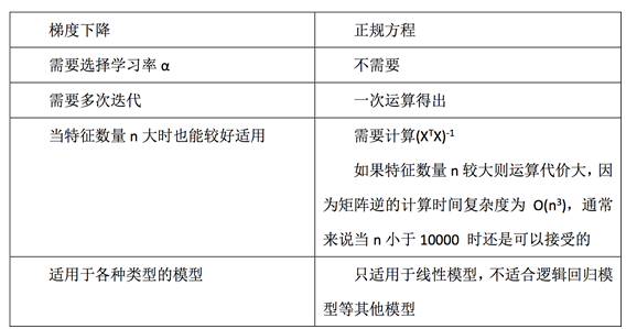
Comparison: Normal Equation vs Gradient Descent

1. Evaluation of LinearRegression and SGDRegressor.
2. Characteristics: Linear regression is the simplest and most user-friendly regression model.
   • It may be limiting, but if we don't know the relationships between features, linear regression is often our first choice.
   • Small datasets: LinearRegression (cannot handle overfitting) and others.
   • Large datasets: SGDRegressor.

Overfitting and Underfitting

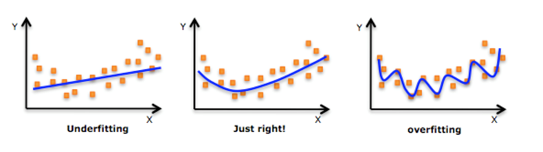
In machine learning, ganeralization refers to the model's performance on unseen samples it hasn't encountered during training. We often discuss overfitting and underfitting. Models are trained and tested on separate datasets. When fitting the training data, we need to consider each point, including noise. If a model learns the details and noise in the training data too well, it may perform poorly on new data. This leads to a complex model with high fitting, causing overfitting. Conversely, if the model only captures part of the data, it's too simple, leading to underfitting, where the model performs poorly on both training and test data.

Illustrations of fitting in linear regression:

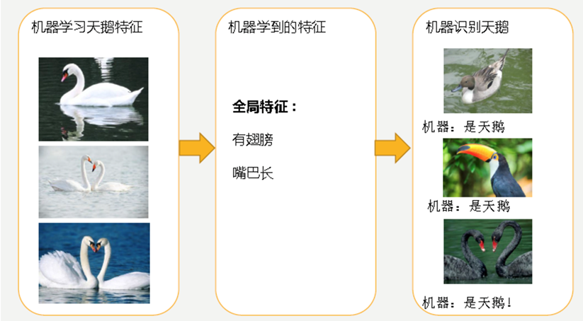
Figure 1 Analysis

After training, the model learned that swans have wings and long beaks. It simply assumes any creature with these features is a swan. The model learned too few features, resulting in a rough criterion that fails to accurately identify swans.

Figure 2 Analysis

The model learned from images to identify swan features: wings, long curved beaks, long slightly curved necks, and a body shape like a "2" slightly larger than a duck. It can now distinguish swans from other animals. However, since all training images were of white swans, the model learned that swans have white feathers. It would then misclassify black swans as non-swans.

Linear models can become complex during training:

Causes and Solutions for Underfitting:

• Cause: Too few features learned.
• Solution: Increase the number of features.

Causes and Solutions for Overfitting:

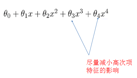
• Cause: Too many original features, including noisy ones; the model is too complex, trying to fit every data point.
• Solutions:
  • Feature selection to eliminate highly correlated features (difficult).
  • Cross-validation (allow all data to be used for training).
  • Regularization (understanding required).

Ridge Regression

Ridge regression is a linear least squares method with L2 regularization. It is a biased estimation regression method specifically designed for collinear data analysis. Essentially, it is an improved least squares estimation method that sacrifices unbiasedness and some information to obtain more realistic and reliable regression coefficients. It is more robust to ill-conditioned data than ordinary least squares. Ridge regression is useful when there is collinearity in the dataset.

• sklearn.linear_model.Ridge(alpha=1.0): Linear least squares with L2 regularization.
  • alpha: Regularization strength.
  • coef_: Regression coefficients.

Comparison: Linear Regression vs Ridge Regression

• Ridge regression: Produces regression coefficients that are more realistic and reliable. It also reduces the fluctuation range of estimated parameters, making them more stable. It has significant practical value in studies with many ill-conditioned data points.

from sklearn import datasets
from sklearn.model_selection import train_test_split
from sklearn.linear_model import RidgeCV
from sklearn.metrics import mean_squared_error

def predict_boston():
    """
    Predict Boston housing prices using ridge regression.
    :return: None
    """
    dataset = datasets.load_boston()
    x_train, x_test, y_train, y_test = train_test_split(dataset.data, dataset.target, test_size=0.2)

    model = RidgeCV(alphas=(1.0, 0.5, 0.01))
    model.fit(x_train, y_train)
    predictions = model.predict(x_test)
    print("Ridge predictions:", predictions)
    mse = mean_squared_error(y_test, predictions)
    print("Ridge MSE:", mse)
    print("Best alpha:", model.alpha_)

if __name__ == '__main__':
    predict_boston()

Output:

Ridge predictions: [25.31 27.01 13.23 27.54 23.74 19.45 13.51 16.47 26.03 20.88 21.12 23.41 13.21 31.15 24.48 15.68 21.31 16.50 16.81 14.59 26.90 25.14 23.10 20.79 13.37 29.02 20.84 17.90 28.36 32.24 25.20 22.19 32.78 28.41 17.21 21.53 15.62 40.93 33.67 17.42 17.95 14.86 37.10 21.78 20.94 21.50 17.73 24.68 45.39 34.52 16.96 30.85 22.63 27.42 38.77 30.05 25.39 27.77 22.17 36.41 27.63 21.19 21.79 24.93 21.29 30.27 34.49 28.61 26.56 34.08  6.27 24.91 20.05 16.35 16.11 17.25  3.71 18.23 16.40 17.59  8.89 15.51 27.71 19.62 16.84 14.33 21.65 20.48 27.12 19.68 30.87 22.29 22.61 24.86 15.07 24.71 22.33 31.40 24.53 16.84 34.42 13.68]
Ridge MSE: 26.83
Best alpha: 0.01

Logistic Regression (Classification Algorithm)

Use Cases:

• Ad click-through rate prediction
• Spam email detection
• Disease diagnosis
• Financial fraud detection
• Fake account detection

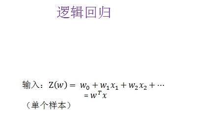
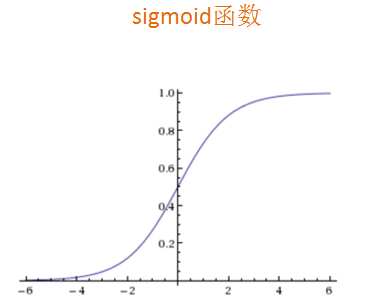
Logistic regression is a powerful tool for binary classification problems.

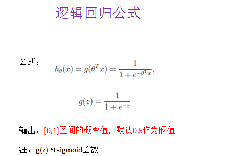
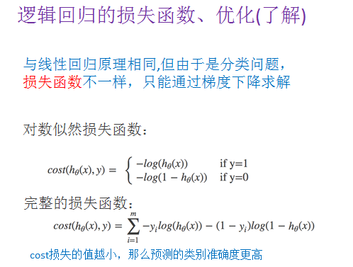
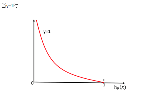
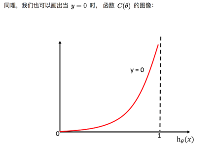
Scikit-learn Logistic Regression API:

• sklearn.linear_model.LogisticRegression()

Case Study: Breast Cancer Prediction

Data Source:

• UCI Machine Learning Repository

Data Description:

• 699 samples, 11 columns. The first column is an ID, the next 9 are medical features related to tumors, and the last column indicates tumor type (benign/malignant).
• 16 missing values are denoted with "?".

from sklearn.model_selection import train_test_split
from sklearn.linear_model import LogisticRegression
from sklearn.metrics import classification_report
import pandas as pd
import numpy as np

def predict_cancer():
    """
    Predict breast cancer using logistic regression.
    :return: None
    """
    columns = ['Sample code number', 'Clump Thickness', 'Uniformity of Cell Size', 'Uniformity of Cell Shape',
               'Marginal Adhesion', 'Single Epithelial Cell Size', 'Bare Nuclei', 'Bland Chromatin',
               'Normal Nucleoli', 'Mitoses', 'Class']
    data = pd.read_csv("https://archive.ics.uci.edu/ml/machine-learning-databases/breast-cancer-wisconsin/breast-cancer-wisconsin.data",
                       names=columns)
    data = data.replace('?', np.nan)
    data = data.dropna()

    X = data[columns[1:10]]
    y = data[columns[10]]

    X_train, X_test, y_train, y_test = train_test_split(X, y, test_size=0.2)

    model = LogisticRegression()
    model.fit(X_train, y_train)

    print("Coefficients:", model.coef_)
    predictions = model.predict(X_test)
    print(predictions)
    accuracy = model.score(X_test, y_test)
    print("Accuracy:", accuracy)
    report = classification_report(y_test, predictions, labels=[2, 4], target_names=["Benign", "Malignant"])
    print(report)

if __name__ == '__main__':
    predict_cancer()

Output:

Coefficients: [[ 0.7081866  -0.11357033  0.21913334  0.34883572 -0.12931481  0.52450199 0.66097954  0.4811952   0.84532057]]
[2 4 4 2 2 4 4 4 2 2 2 4 4 2 2 2 4 4 2 4 2 2 2 2 4 2 2 2 2 4 2 4 2 4 2 4 4 4 4 2 2 4 2 4 4 2 4 2 2 2 4 2 4 2 2 2 2 2 4 2 4 2 2 2 4 2 2 4 2 4 2 2 2 2 4 4 2 2 2 2 2 4 4 2 4 4 4 2 4 2 4 4 4 4 2 4 4 2 2 4 2 2 2 2 2 2 4 2 4 4 2 2 4 2 4 2 2 2 4 2 4 2 2 2 2 2 4 4 4 4 2 2 2 2 4 2 2]
Accuracy: 0.9635036496350365
              precision    recall  f1-score   support

     Benign       0.96      0.97      0.97        80
  Malignant       0.96      0.95      0.96        57

    accuracy                           0.96       137
   macro avg       0.96      0.96      0.96       137
weighted avg       0.96      0.96      0.96       137

Logistic Regression Summary:

• Applications: Ad click-through rate prediction, e-commerce product recommendations.
• Advantages: Suitable for scenarios requiring classification probabilities, simple, fast.
• Disadvantages: Handles multi-class problems poorly.

Unsupervised Learning

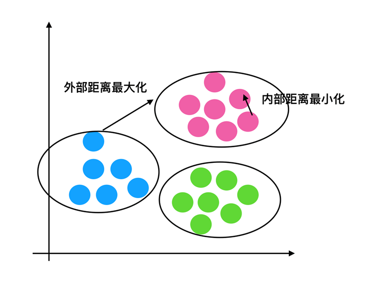
Unsupervised learning, as the name suggests, is a free learning method without supervision. It does not require prior knowledge for guidance but continuously self-learns, self-consolidates, and self-summarizes. In machine learning, unsupervised learning can be simply understood as not providing corresponding class labels for the training set.

"Birds of a feather flock together."

K-Means Clustering

K-means, often called Lloyd's algorithm, is one of the most classic and easily understood models in data clustering. The algorithm execution process has four stages:

1. Randomly set K points in the feature space as initial cluster centers.
2. For each data point, find the nearest cluster center among the K centers and assign the point to that cluster.
3. After all points are assigned, recalculate cluster centers by taking the mean of all points in each cluster.
4. Compute the difference between old and new centers. If no data point changes its cluster assignment, the iteration stops; otherwise, return to step 2.

K-means is equivalent to the expectation-maximization algorithm with small, full covariance matrices.

K-Means API:

• sklearn.cluster.KMeans(n_clusters=8, init='k-means++')
  • n_clusters: Number of initial cluster centers.
  • init: Initialization method, default is 'k-means++'.
  • labels_: Default label type, can be compared with true values (not direct value comparison).

K-Means Performance Evaluation API:

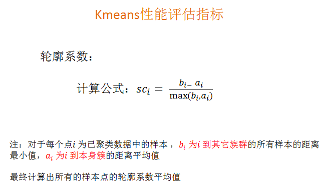
• sklearn.metrics.silhouette_score

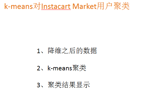
K-Means Case Study

import pandas as pd
from sklearn.decomposition import PCA
from sklearn.cluster import KMeans
from matplotlib import pyplot as plt
from sklearn.metrics import silhouette_score

orders = pd.read_csv("./data/instacart/orders.csv")
aisles = pd.read_csv("./data/instacart/aisles.csv")
order_products_prior = pd.read_csv("./data/instacart/order_products_prior.csv")
products = pd.read_csv("./data/instacart/products.csv")
merged = pd.merge(orders, order_products_prior, on=['order_id','order_id'])
merged = pd.merge(merged, products, on=['product_id', 'product_id'])
merged = pd.merge(merged, aisles, on=['aisle_id','aisle_id'])
# User and product category relationship
cross_tab = pd.crosstab(merged['user_id'], merged['aisle'])

# PCA for dimensionality reduction
pca = PCA(n_components=100)
reduced_data = pca.fit_transform(cross_tab)
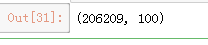
reduced_data.shape

x_train = reduced_data[:1000]
x_test = reduced_data[1000:1300]

km = KMeans(n_clusters=4)
km.fit(x_train)

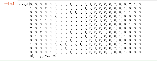
predictions = km.predict(x_test)
predictions

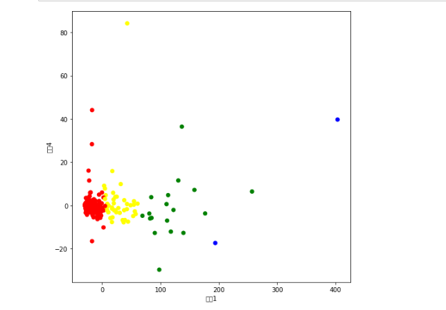
plt.figure(figsize=(8,8))
colors = ["red","yellow","green","blue"]
colored = [colors[i] for i in predictions]
plt.scatter(x_test[:, 0], x_test[:, 4], c=colored)
plt.xlabel("Feature 1")
plt.ylabel("Feature 4")
plt.show()

silhouette_score(x_test, predictions)