Reference Book: [1] Clifford A. Shaffer. Data Structures and Algorithm Analysis[M]. Beijing: Electronic Industry Press, 2020.

Data Structures and Algorithms

Problems, Algorithms, and Programs

Q: What can be called an algorithmm?

1. It must be correct.
2. It is composed of a series of concrete steps.
3. It is unambiguous.
4. It must be composed of a finite number of steps.
5. It must terminate.

Mathematical Preliminaries

Logarithms

If (\log_2 x = y), then 2 can be omitted: (\log x = y).

Algorithm Analysis*

Asymptotic analysis attempts to estimate the resource consumption of an algorithm.

Introduction

Growth rate: (2 < \log_2 x < n^{2/3} < n < n^2 < 3^n < n!)

Asymptotic Analysis

Upper Bounds: (O(g(n))) Lower Bounds: (\Omega(g(n))) When upper and lower bounds are the same: (\Theta(g(n)))

Simplifying Rules

1. Omit constant coefficients: (\Theta(kg(n)) = \Theta(g(n)))
2. Take highest-order term: (\Theta(g(n) + f(n)) = \Theta(\max(g(n), f(n))))

Calculating the Running Time for a Program

1. sum = 0; Assignment: (\Theta(1))
2. for (i = 1; i <= n; i++) { sum += n; } Loop: (\Theta(n))
3. Nested loops (multiply inner and outer layers): (\Theta(n \log n))

for (i = 1; i <= n; i *= 2)
    for (j = 1; j <= n; j++)
        sum++;

Lists, Stacks and Queues

Linear Lists

Linear lists have a unique head and tail, with data in order. <20, 23 | 12, 15>: current element is 12, current position is 2.

Array-based Lists

All data is stored sequentially.

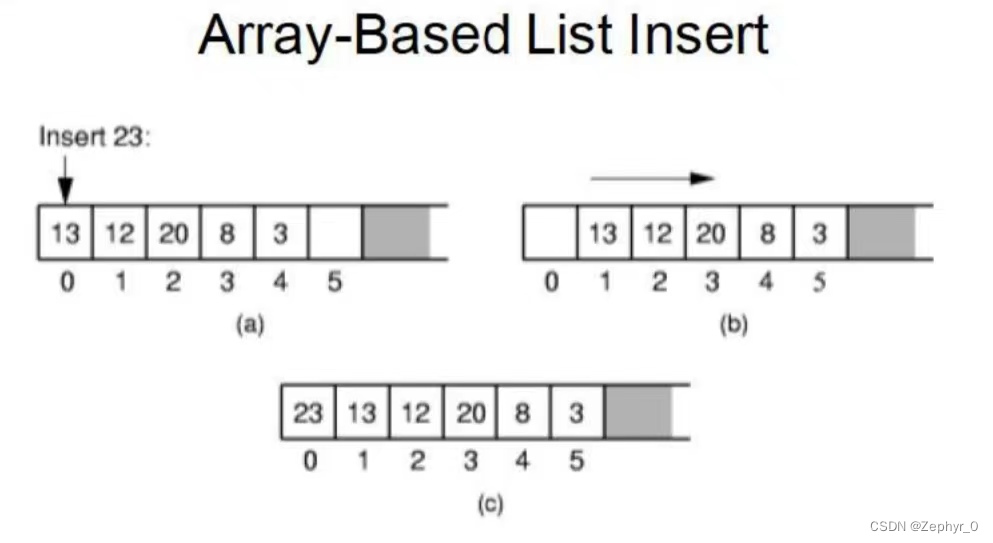
Insert Data

for (int i = listSize; i > curr; i--)
    listArray[i] = listArray[i - 1];

Shift data backward to make space: (\Theta(n))

Performance of Array-based Lists (\Theta(n)): Insert, delete (remove), and locate (\Theta(1)): Clear, empty, full, length, replace, get, prev (move one step forward from current position)

Linked Lists

Data can be stored non-contiguously and can be expanded.

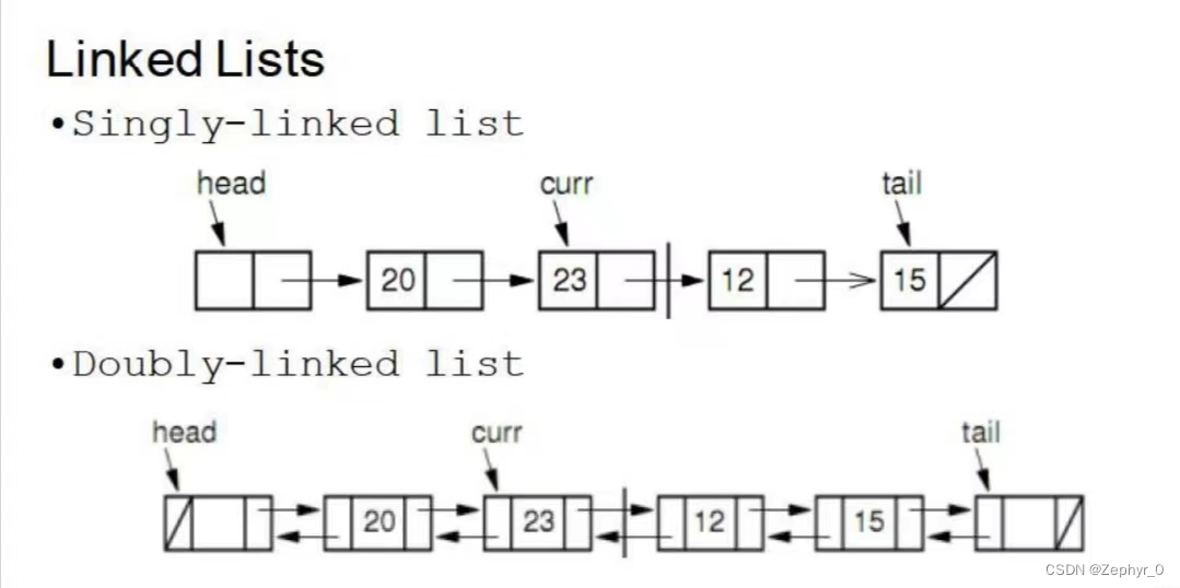
Linked lists consist of nodes, where Node = element + next (element and pointer).

Singly Linked List Includes a header node at the front of the list, which does not store data, simplifying list operations. Tip: Inserting an element at curr is not the same as inserting at position i (the former inserts directly, the latter requires searching from the head to find position i).

Insert New Element x at the i-th Node of the Linked List

if (head == NULL || i == 0) { // Insert at front
    newNode->next = head;
    if (head == NULL) tail = newNode; // Originally empty list
    head = newNode; // Transfer header
} else { // Insert in middle or at tail
    newNode->next = p->next;
    if (p->next == NULL) tail = newNode;
    p->next = newNode; // Change two pointers to insert new node
}

Performance of Singly Linked List (\Theta(1)): Insert, delete (remove) (\Theta(n)): Prev (move one step forward from current position), direct access

Space Comparison n: Number of elements in the list E: Space occupied by each data element P: Space occupied by each pointer D: Maximum number of elements the list can have When DE < n(P + E), Singly Linked List has lower storage efficiency than Array-based Lists.

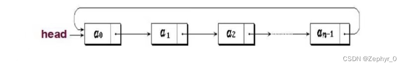
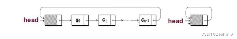
Circular List The next pointer of the last node points to the front of the list.

Doubly Linked Lists Compared to singly linked lists, adds a forward pointer, solving the inconvenience of moving forward in singly linked lists. However, more pointers mean more storage space is needed to store them.

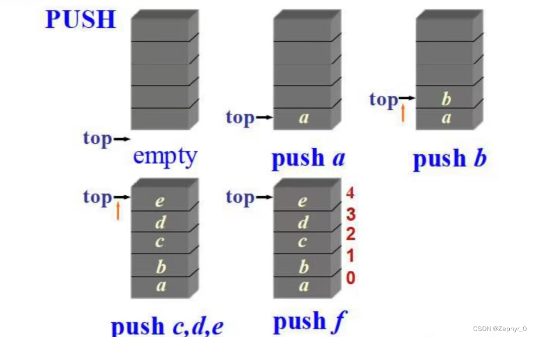
Stacks

Last-In-First-Out (LIFO) linear list (including linear lists and linked lists). The top of the stack is at the tail of the linear list (i.e., push and pop are equivalent to insert and remove at the tail of the linear list).

Push (if too many are added, overflow occurs)

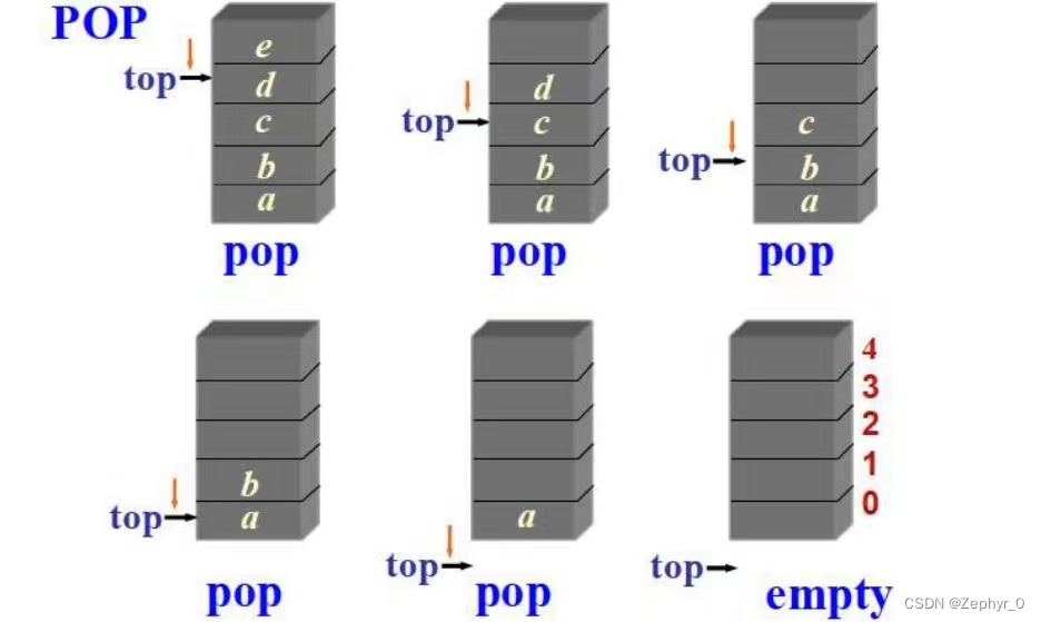
Pop (if too many are removed, underflow occurs)

Stack Application Function nesting, recursion, etc.

Queues

First-In-First-Out (FIFO) linear list, with front head and rear tail.

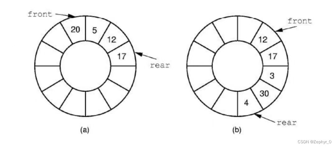
Empty queue: rear == front Full queue: (rear + 1) % maxSize == front

Binary Tree

Definition

Node Subtree - left and right subtrees are different Degree - number of subtrees of a node, binary tree degree (\leqslant 2) Children - child nodes Parent - parent node Edge Path - from (n_1) to (n_k) Length - path length (k - 1) Ancestor (multiple) Descendant (multiple) Depth - root is 0, increasing by 1 downward Height - number of layers of the tree Leaf node - node without descendants Internal node - node with descendants Sibling node - nodes with the same parent

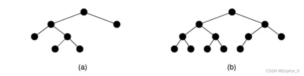
Full binary tree - if there are subtrees, there must be two (a) Complete binary tree - all layers except the last are full, last layer filled from left to right (b)

Theorem Leaf node ((n_0)) = internal node ((n_2)) + 1 (holds for all full binary trees) Inference: Number of empty subtrees in a non-empty binary tree = number of nodes + 1

Binary Tree Traversals

Traversal Methods

Abbreviate binary tree nodes: N-root, L-left child, R-right child Traversal methods:

1. Preorder: NLR, NRL
2. Inorder: LNR, RNL
3. Postorder: LRN, RLN (all based on N)

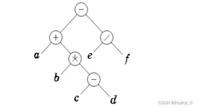
Draw a binary tree: (a + b * (c - d) - e / f) (last computed at the root)

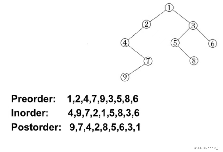
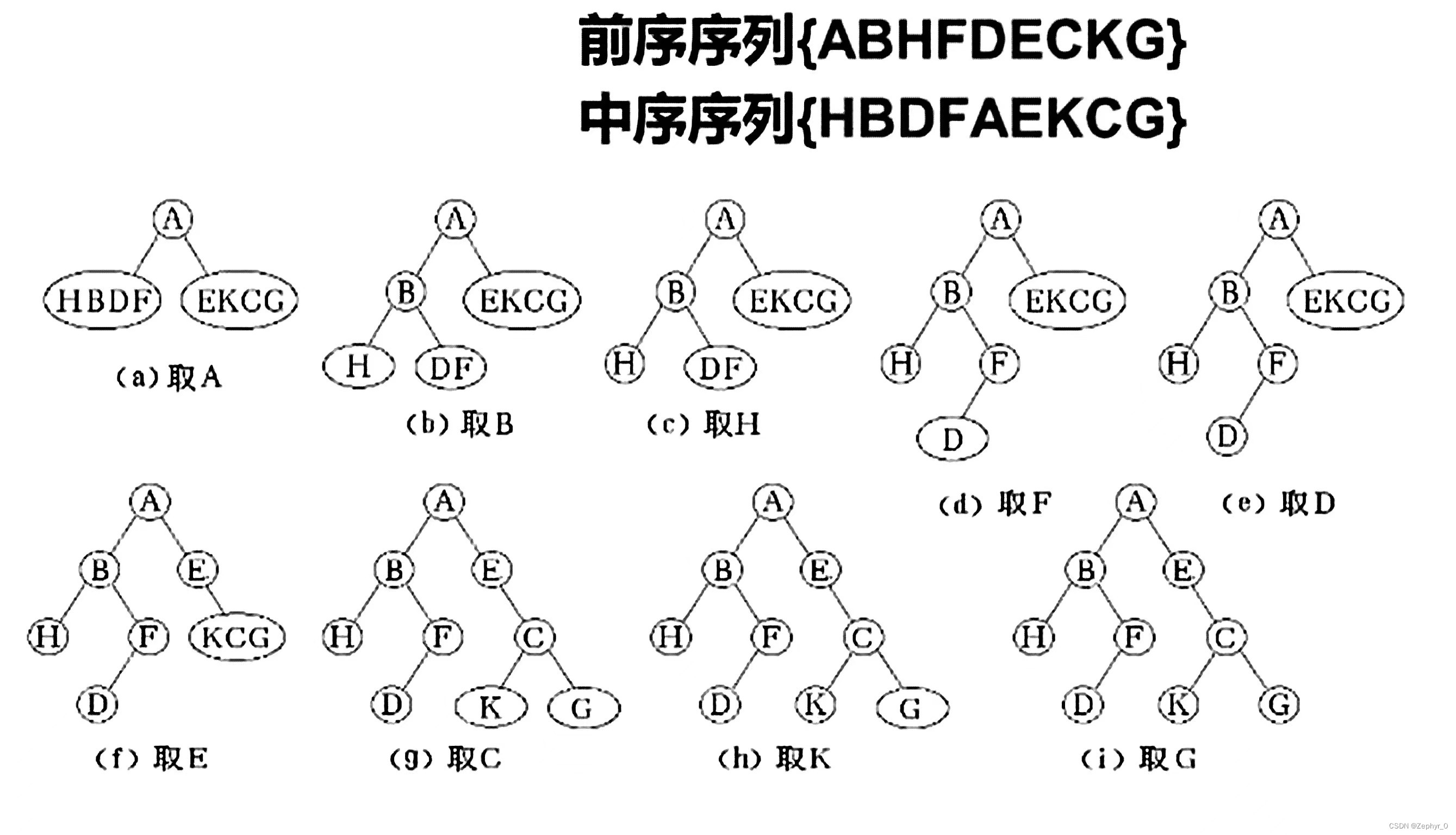
Restoring Binary Tree from Traversal Sequences

Preorder and inorder, or postorder and inorder can uniquely determine a binary tree.

Binary Tree Node Implementations

Internal node IntlNode includes element and two pointers, pointing to leftChild and rightChild respectively. Leaf node LeafNode only includes element. (Binary tree implementation and traversal code can be found in the data structures and algorithms code section.)

Binary Search Tree (BST)

Binary search tree elements are placed in increasing order, satisfying leftChild < root (\leqslant) rightChild.

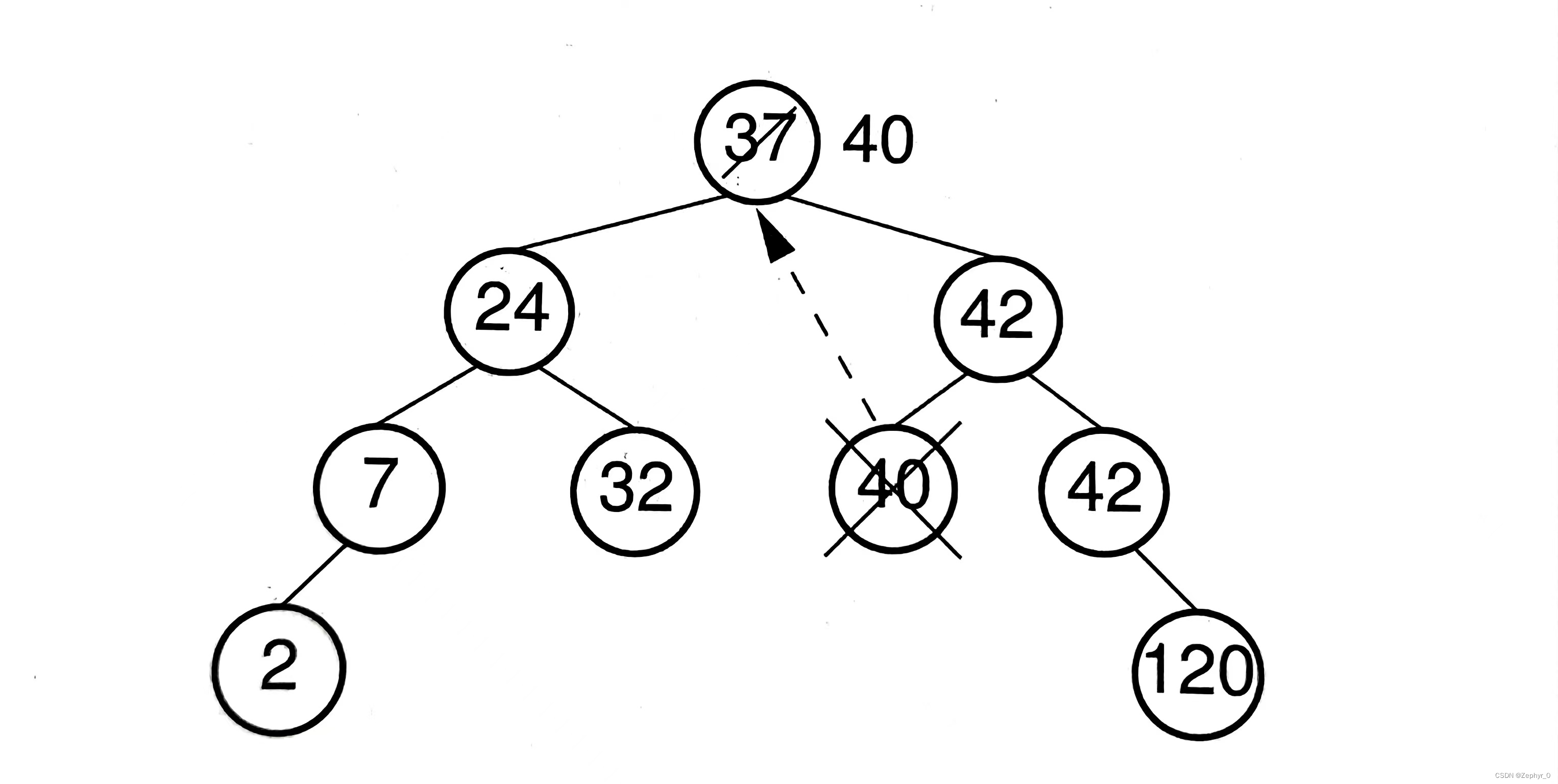
Remove Function (1) 0 children: leaf node, remove directly (2) 1 child: remove the node and move the child node up (3) 2 children: find a node to replace this node, generally choose the smallest node on the right or the largest node on the left

When the search tree is relatively balanced, the time complexity of the remove function is (\Theta(\log n)), where (n) is the depth of the tree.

(BST code can also be found in the data structures and algorithms code section.)

Heaps and Priority Queues

Heap is a complete binary tree, divided into max-heap (root greater than two child nodes) and min-heap (root less than two child nodes).

Siftdown Algorithm: When a node does not meet the condition, compare and swap positions with left and right child nodes, then continue comparing with child nodes.

void siftdown(int pos) {
    while (!isLeaf(pos)) { // Stop if pos is a leaf
        int j = leftChild(pos);
        int rc = rightChild(pos);
        if ((rc < n) && Comp::prior(Heap[rc], Heap[j]))
            j = rc; // If right child exists and its value has priority over left child, update j to right child position
        if (Comp::prior(Heap[pos], Heap[j]))
            return; // If element at position pos has priority over element at position j, no swap needed, function returns
        swap(pos, j); // Move down
        pos = j;
    }
}

When the heap is relatively balanced, the time complexity of insert, delete, and find element functions is (\Theta(\log n)), where (n) is the depth of the tree.

(Max-heap implementation code can also be found in the data structures and algorithms code section.)

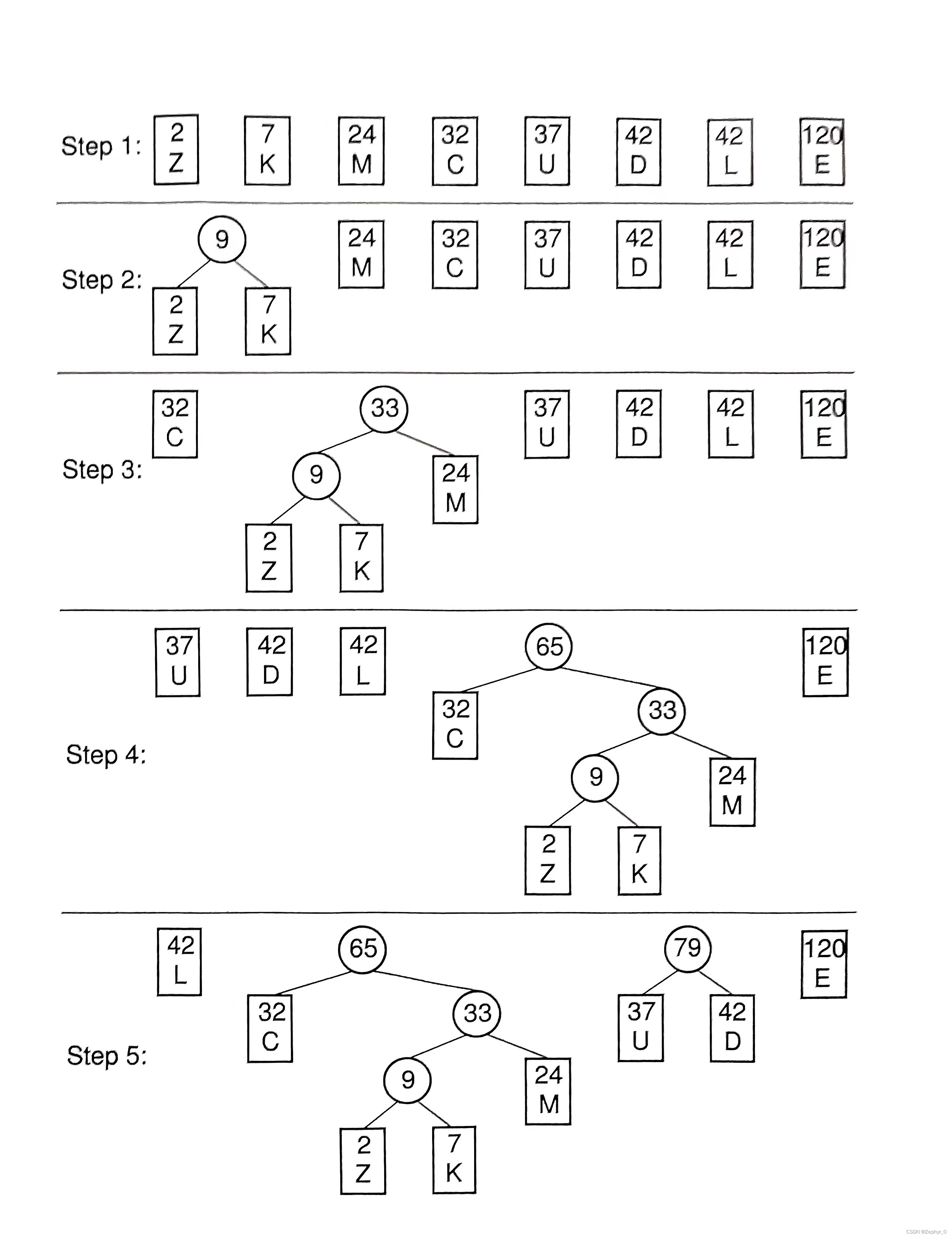
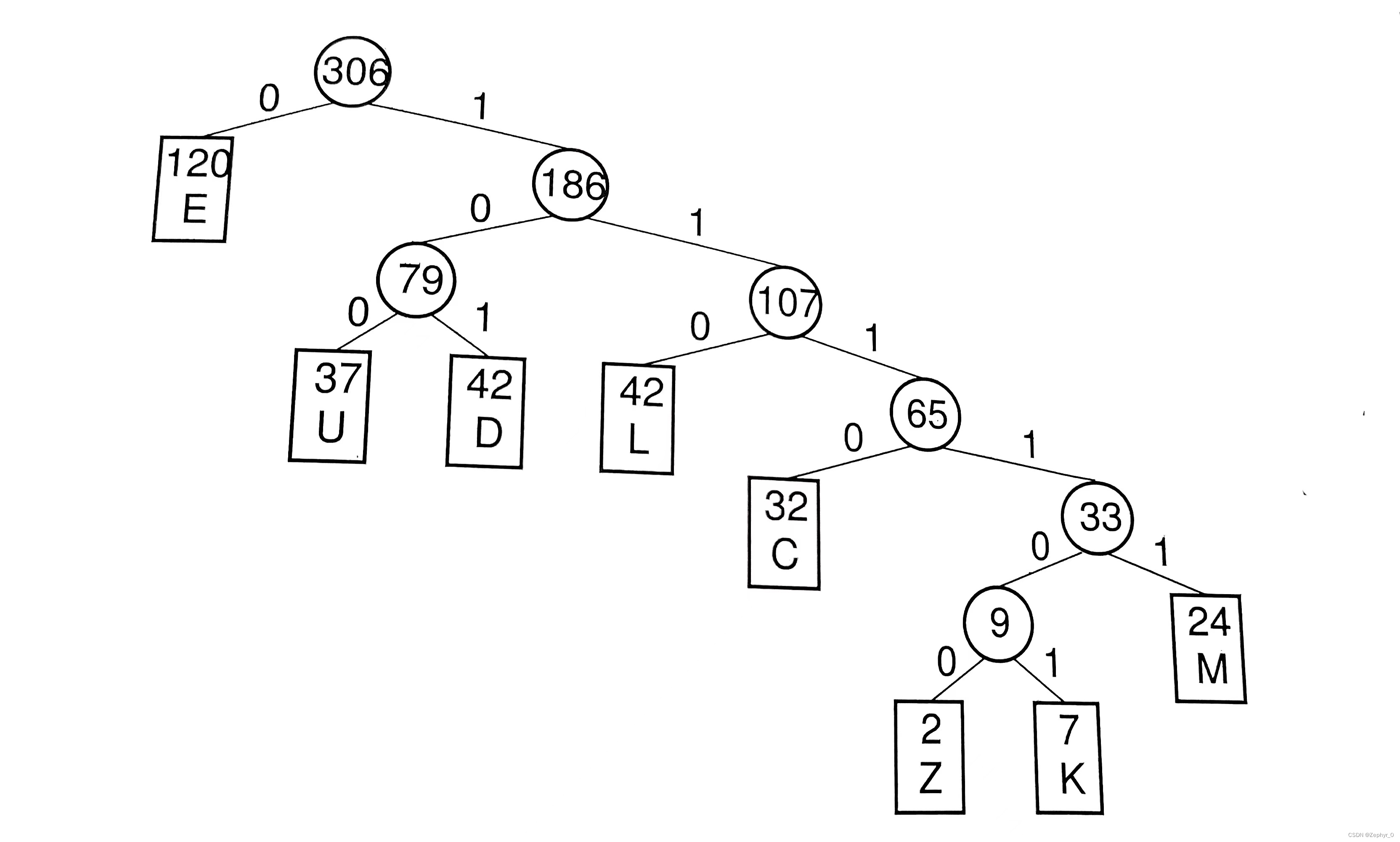
Huffman Coding Trees

Weighted path length External path weight Encoding Steps:

(Huffman coding tree implementation code can also be found in the data structures and algorithms code section.)

Non-Binary Trees

Forest: one or multiple trees

ADT for Nodes and General Tree Traversals

Nodes are similar to binary trees, adding sibling (same parent node).

// General tree node ADT
template <typename E>
class GTNode {
public:
    E value();
    bool isLeaf();
    GTNode* parent();
    GTNode* leftmostChild();
    GTNode* rightSibling(); // Return right sibling
    void setValue(E&);
    void insertFirst(GTNode<E>*); // Insert first child
    void insertNext(GTNode<E>*); // Insert next sibling
    void removeFirst();
    void removeNext();
};

Traversal: Only preorder and postorder traversals.

The Parent Pointer Implementation

Advantages

Parent Pointer: pointer from child node to parent node Advantages: (1) Determine if two nodes are in the same tree (find ancestor nodes, if ancestors are the same then in the same tree) (2) Merge two trees (directly attach the root of one tree to the root of another tree)

Classes and Union-Find

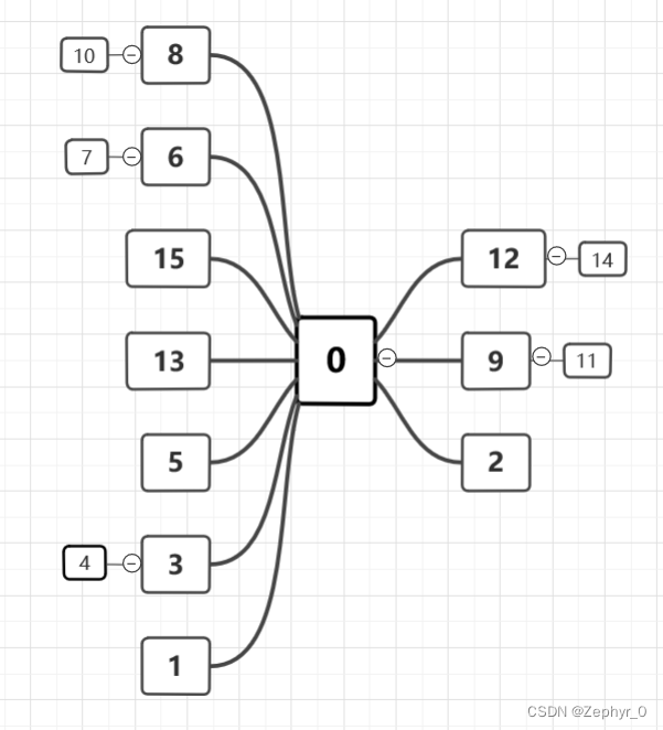
Classes and Union-Find includes weighted union rule and path compression Example: Using the weighted union rule and path compression, show the array for the parent pointer implementation that results from the following series of equivalences on a set of objects indexed by the values 0 through 15. Initially, each element in the set should be in a separate equivalence class. When two trees to be merged are the same size, make the root with greater index value be the child of the root with lesser index value. (0,2) (1,2) (3,4) (3,1) (3,5) (9,11) (12,14) (3,9) (4,14) (6,7) (8,10) (8,7) (7,0) (10,15) (10,13) Solution

1. Problem requires smaller number above larger number (pointer from larger number to smaller number)
2. Add sequentially, performing compression while adding When merging (x,y) (e.g., (4,14)), first find the roots of x and y respectively, compare root sizes, if root(x) > root(y), point root(x) to root(y), merging the two trees.

General Tree Implementasions

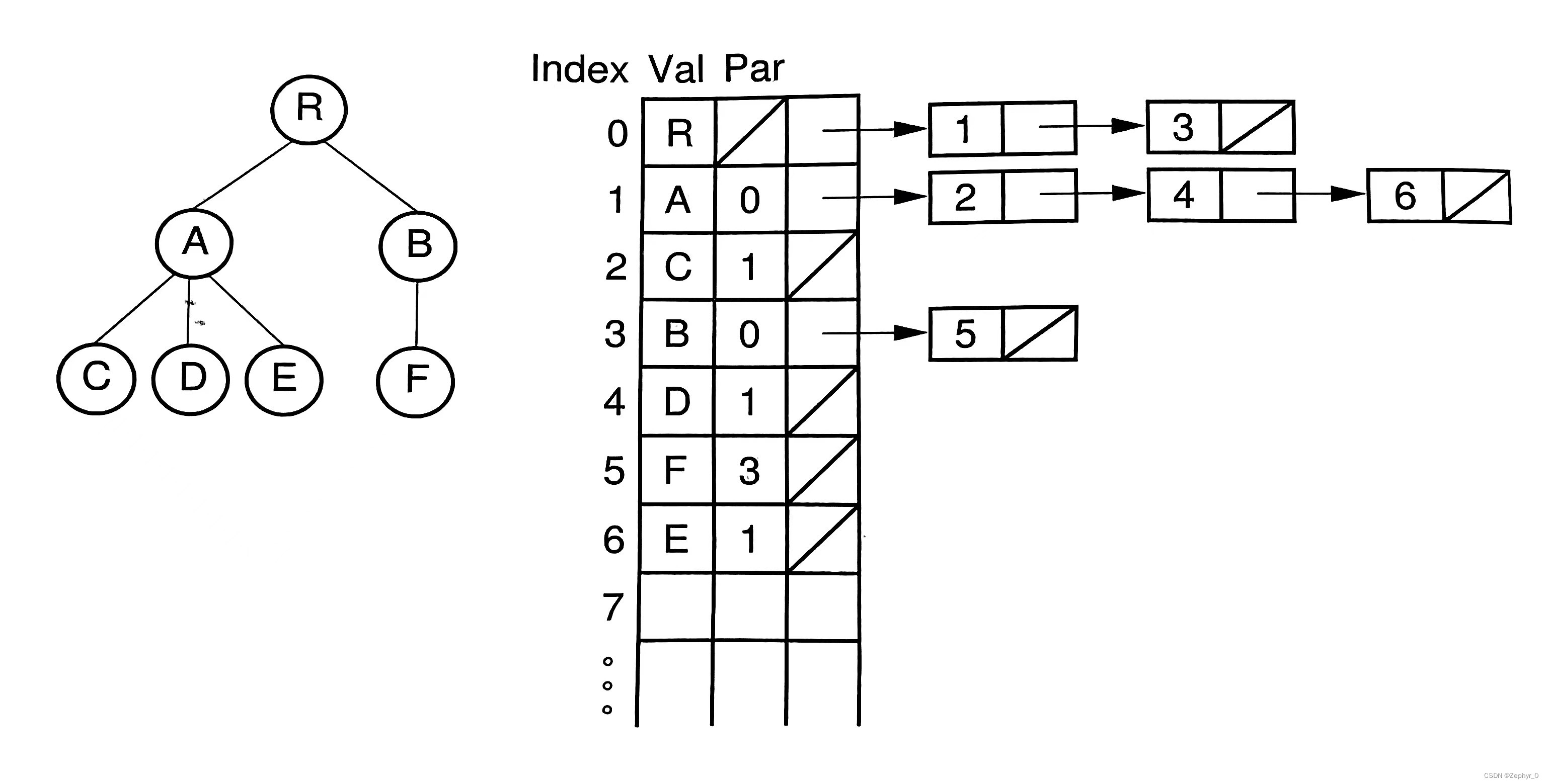
(The following implementations have no code, only diagrams.) 1. List of Children Represantation Val: Node name Par: Index value of parent node

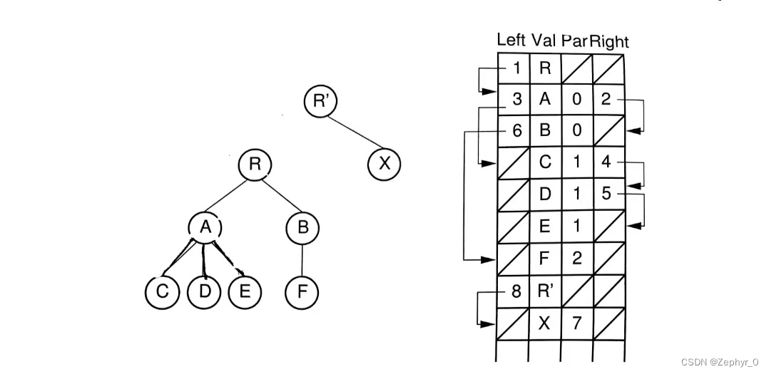
2. Left-Child/Right-Sibling Representation Left: Pointer to leftmost child node position Right: Pointer to first sibling node position on the right

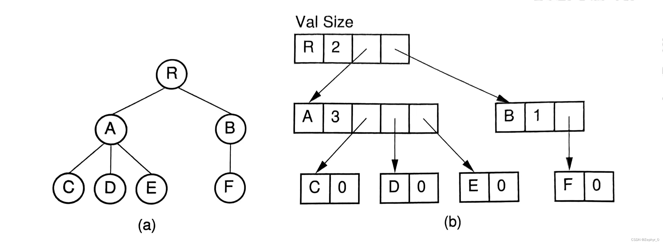
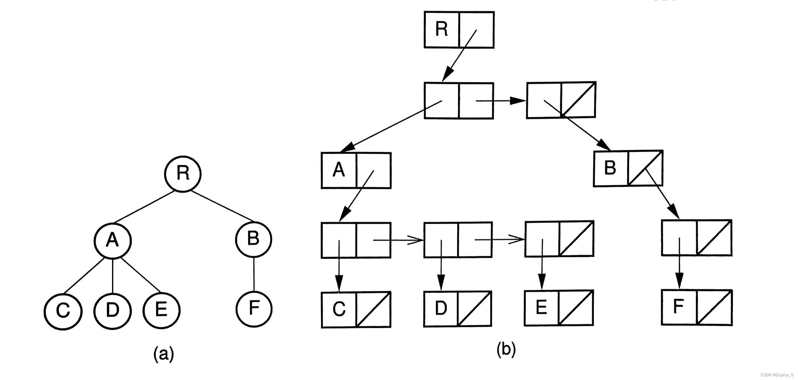
3&4. Two Dynamic Node Representations

K-ary Trees

Similar to binary trees, divided into Full k-ary trees and Complete k-ary trees.

Sequential Tree Implementations

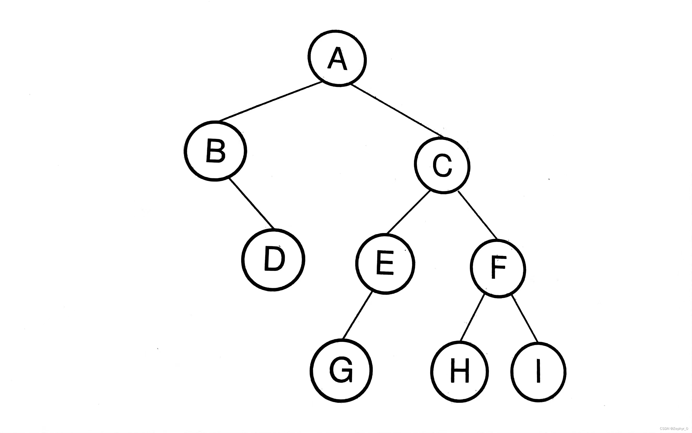
1. Use / to represent empty nodes (AB/D//CEG///FH//I//) 2. Use ' to represent internal nodes, / to represent empty nodes (A'B'/DC'E'G/F'HI) 3. Use ) to represent moving back one step to parent node <ABD))CEG))FH)I)))> does not distinguish left and right nodes